PICWave

Semiconductor Optical Amplifier (SOA)

Simulation with PICWave and Harold software

PICWave can be used in combination with Harold to model an semiconductor optical amplifier (SOA) in the time-domain. The hetero-structure of the SOA will first be modelled in Harold, which will produce a set of material gain curves at different carrier densities. These gain curves will then be exported into PICWave in which the semiconductor optical amplifier will be modelled in 3D in the time domain.

Calculations of the gain curves in Harold
Importation and fitting of the gain curves in PICWave
Amplified Spontaneous Emission (ASE) in the SOA
Gain saturation of the SOA
Dynamic behaviour in the time domain
Four-wave mixing

Calculations of the gain curves in Harold

Harold is a hetero-structure model, which allows you to model the physics of your SOA in great detail. Harold can simulate single and multiple quantum-well structures thanks to a state of the art capture/escape model for carriers in the quantum well. In this case, an InGaAsP-InP hetero-structure is simulated, with four quantum wells.

Hetero-structure defined in Harold

Harold is used to generate gain curves at different carrier densities for the gain material in this hetero-structure. The user can define the range of temperature and carrier density required for the PICWave simulation.

Gain curves at different carrier concentrations calculated in Harold

Importation and fitting of the gain curves in PICWave

These gain curves for the hetero-structure are now imported by PICWave, which will simulate the SOA in 3D in the time domain. The epitaxial structure defined in Harold is also imported and extended into a ridge waveguide.

The gain curves need to be fitted in order to be used by the time domain model. This is done in PICWave using a Wide-Band Gain Fitting. The Wide-Band Gain Fitting allows you to maintain the accuracy of the fitted curves over a very wide range of wavelength. You can see here in comparison the fitted gain curves obtained with a parabolic gain fitting, for which the fitting is only valid near the gain peak.

(a)                                                             (b)

Imported gain curves (green) and fitted gain curves (blue) plotted against wavelength for different carrier densities
(a) with a parabolic gain fitting (b) with the Wide-Band Gain Fitting.

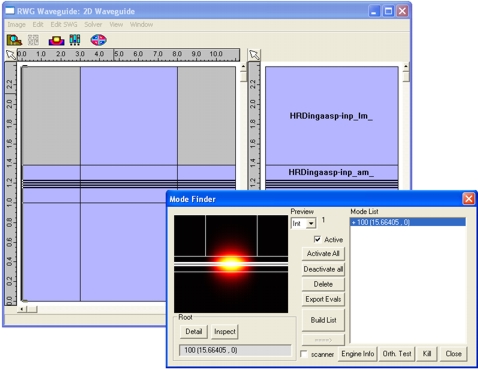
For laser modelling, most of the light is emitted near the peak, and the parabolic gain fitting would be acceptable. For an SOA however an accurate fit over a wide range of wavelength is crucial as the response of the device will be broadband.

Amplified Spontaneous Emission (ASE) in the SOA

The SOA is modelled in 3D in PICWave. The epitaxial structure defined in Harold is used here to define the geometry of the XY cross-section of a ridge waveguide, which will extend over a length of 1mm in the Z-direction.

A fully vectorial FDM mode solver, relying on a finite-difference method, is used to calculate the optical modes of the waveguide. The properties of the optical modes can be calculated in great detail: effective index, propagation constant, optical losses, confinement factor, polarisation, dispersion, etc.

Waveguide-cross section and mode profile for the fundamental TE-like mode
calculated with the fully vectorial FDM Solver

We will first simulate the amplified spontaneous emission (ASE) in the SOA. The SOA is modelled in the time-domain with a constant current drive. You can see here the output power emitted by ASE and the carrier density in the centre of the SOA stabilising after 1ns.

(a)                                                             (b)

Evolution of (a) the output power and (b) the carrier density in the centre of the SOA
in the time-domain at constant current drive

PICWave allows you to explore the spatial profile of the carrier density in the SOA laterally and longitudinally.

The longitudinal z-profile of the carrier density is shown below. The z-profile of the carrier density can be related to the mode intensity profile due to ASE in the SOA. The high optical power is associated with a drop in the carrier density due to stimulated emission.

(a)                                                             (b)

Evolution along the z-axis of the SOA of
(a) the carrier density at the centre of the SOA and
(b) the forward (green), backward (red) and total optical power

You can also study the lateral profile of the carrier density at different positions along the length of the SOA. This allows you to observe effects such as lateral hole burning.

Lateral profile of the carrier density at the end of the SOA.
The dip in the carrier density is due to lateral hole burning.

PICWave features a Lorentzian noise model, which allows you to model the noise spectrum more realistically in the case of a broad free spectral range. The two graphs below show the effect of the noise spectrum on the output spectrum of the SOA driven at the transparency current.

(a)                                                             (b)

Output spectrum of the SOA modelled with (a) a white noise model (b) a Lorentzian noise model
driven at the transparency current.

Gain saturation of the SOA

PICWave allows you to study the gain saturation of the SOA. The gain saturation gives a non-linear response to the output power when the input power is increased above a certain level. It is studied here by measuring the optical output power when the input power is varied between 0 and 5 mW.

The plot of output power against input power below allows us to clearly distinguish the linear (greyed) and the non-linear responses.

Gain saturation: output power as a function of input power (in mW)

It is characterised below by showing the evolution of the ratio of the output to the input power (in dB) as a function of input power (in mW). The linear response corresponds to a horizontal line and is greyed on the plot below.

Gain saturation: ratio of output power / input power (in dB) against output power (in mW)

Dynamic behaviour in the time domain

Dynamic behaviour can also be studied. Here we inject a high-energy optical pulse at constant drive current, which suddenly puts the SOA into the saturated-gain regime. The resulting dip in the carrier density is shown plotted against time.

(a)                                                             (b)

Time-domain response of the SOA to the injection of a high-energy optical pulse at constant drive current:
(a) input pulse and (b) carrier density plotted against time.

Four-wave mixing

PICWave allows you to model other effects in SOAs such as four-wave mixing. In the time-varying power density spectrum measured at the output of an SOA plotted below, only the power at 0nm, 1nm and 4nm has been injected. The power emitted at the other wavelengths is due to four-wave mixing.

Time-evolving spectrum showing four-wave mixing